
Key Takeways:
- Mastering advanced Excel productivity skills like PivotTables, VLOOKUP, and Conditional Formatting can significantly boost workplace productivity and decision-making.
- Real-world examples demonstrate how tools like SUMIF and Data Validation solve practical challenges across sales, HR, and operations.
- Whether you’re upskilling or switching careers, building Excel expertise with structured training such as James Cook Institute’s Excel WSQ accredited courses gives you an edge in today’s data driven job market.
While basic Excel skills such as data entry, simple formulas, and chart creation are essential starting points, they’re often not enough in roles that demand advanced Excel functions, workplace data analysis, or more complex Excel reporting techniques, especially when working with larger datasets and making data-driven decisions.
As your responsibilities grow, so does the complexity of the tasks you’re expected to manage, and that’s where advanced Excel skills become critical.
Mastering advanced Excel techniques can make your day-to-day tasks more efficient, streamline decision-making, and significantly enhance your overall productivity. These skills are not only practical for the workplace, but also powerful additions to your resume, giving you a competitive edge in today’s fast-paced job market.
Whether you’re working in finance, data analytics, marketing, operations, or administration, the ability to confidently navigate advanced Excel functions can open up new career opportunities and fast-track your professional growth.
Here are 5 advanced Excel skills that will help you work with improved efficiency, streamline data analysis, and boost your overall workplace productivity.
- Pivot Table & Pivot Chart
- VLOOKUP, HLOOKUP
- Conditional Formatting
- CountIF & sumIF
- Data Validation
Pivot Table & Pivot Chart
PivotTables are a powerful Excel feature that lets you summarise, analyse and explore large sets of data, making them one of the most effective Excel reporting techniques available.
- It groups and totals your data automatically (e.g. sales by staff, revenue by quarter, item counts by category).
- You can filter, sort, and rearrange the layout to see your data from different angles.
- PivotTables help you turn messy rows into clear, actionable summaries with just a few clicks.
Whether you’re in sales, finance, HR, or operations, PivotTables help you uncover trends, generate reports, and answer questions fast, making them ideal for decision-making and stakeholder reporting.
Pivot Table Use Case Example
You’re tracking sales across multiple staff, products, and time periods.
Each row in your spreadsheet logs a single sale with the staff member’s name, the sport sold, the quarter it occurred in, and the amount.
Now you’re asked questions like:
- How much did each staff member sell in each quarter?
- Which sports are bringing in the most sales?
- How many transactions did each person handle?
That’s where Pivot Table comes in:
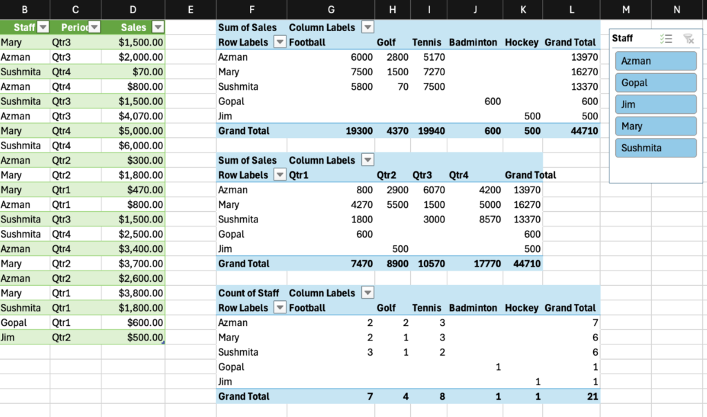
In this example:
- The first PivotTable shows total sales by staff and sport
- The second one breaks down sales by staff across all four quarters
- The third counts how many times each staff sold each sport
The filter panel on the right lets you toggle visibility instantly, no formulas needed. With just a few clicks, PivotTables turn raw rows of data into dynamic summaries, helping you uncover patterns and insights fast.
VLookup & HLookup
VLOOKUP and HLOOKUP are lookup functions in Excel that help you search for specific data within a table.
- VLOOKUP (vertical lookup) searches down the first column of a table and returns a value from the same row.
- HLOOKUP (horizontal lookup) searches across the first row and returns a value from the same column.
These functions are useful for retrieving information quickly without manually scanning through large datasets.
HLookup Use Case Example
magine you’re managing a class of 20 students and you’ve calculated each student’s percentage based on their total marks. Now, you need to assign letter grades : A, B, C, D, or F – based on those percentages.
You could go through each student manually and match their score to a grading scale, but what happens when there are hundreds of students? Or if the grading scale changes later?
That’s where HLOOKUP comes in.
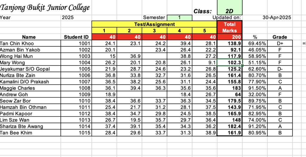
What is the formula doing:?
=HLOOKUP(1, C4:G5, 2, FALSE) looks across the assignment numbers in row 4, finds Assignment 1, and returns the full mark from the row below – in this case, 40.
This helps automate grading. Instead of hardcoding the full mark, the formula dynamically pulls it. So, if full marks change, the calculations update automatically. It’s useful for percentage calculations and keeping the sheet flexible.
VLookup Use Case:
Let’s say you’re managing an inventory sheet and need to find the price of an item based on its Product ID. Instead of scanning through a long product list, you can use VLOOKUP.
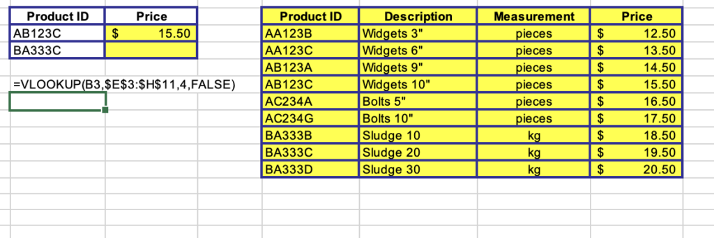
In this case, the formula =VLOOKUP(B3, $E$3:$H$11, 4, FALSE) searches for the Product ID entered in cell B3, scans the product list, and returns the corresponding price from column 4. automatically. It saves time, avoids mistakes, and keeps your price list dynamic and scalable.
Conditional Formatting
Conditional Formatting automatically highlights important data trends by applying colours, icons, or data bars based on rules you set. It allows you to visualise problems, risks, and opportunities instantly – such as flagging overdue projects, spotting underperforming departments, or highlighting top-performing salespeople.
Conditional Formatting Use Case Example:
You’re working with a large dataset that tracks product sales, event dates, and student progress.
You need to:
- Spot duplicate entries or outlier values
- Compare performance numbers quickly
- Instantly identify whether students improved after training
You could scroll through hundreds of rows manually, scanning for mistakes and calculating performance changes, but that’s time-consuming and prone to error.
That’s where Conditional Formatting comes in.
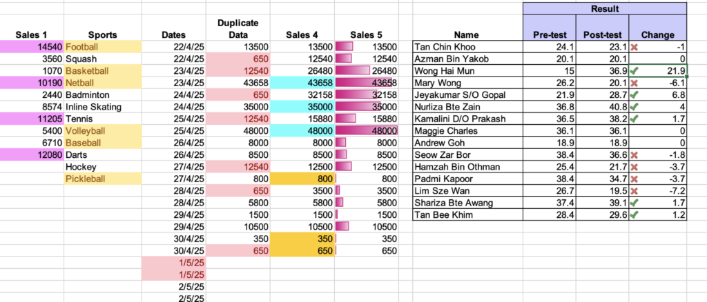
In this example, duplicate entries and data issues are automatically flagged in red, allowing you to catch errors immediately. Sales performance is visualised using data bars, making it easy to compare figures without scanning every number. And when it comes to student progress, checkmarks and crosses quickly show who improved and who didn’t
Data Validation
Data Validation restricts the type of data that can be entered into a cell, for example, limiting input to whole numbers, enforcing dropdown selections, or ensuring that text matches a specific format like an email address.
It can also be used to:
- Create dropdown menus
- Prevent duplicate entries
- Flag invalid formats (e.g. typos in emails)
- Standardise data across teams using predefined rules
Data Validation helps maintain clean, accurate, and consistent datasets, especially in shared workbooks. It reduces manual errors, prevents formatting issues, and ensures only valid entries are allowed, which is crucial for accurate reporting and analysis.
Data Validation Use Case Example:
You’re managing customer orders, and you want to make sure that every delivery date entered falls within a reasonable window, specifically, within 7 days of the order date. You could manually check every row, but what if you’re dealing with hundreds of orders and multiple users filling out the sheet?
That’s where Data Validation comes in
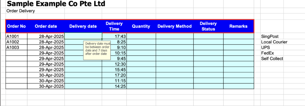
This sheet uses a custom data validation rule to ensure delivery dates are within 7 days of the order date. A tooltip guides the user with the message:
“Delivery date must be between order date and 7 days after order date.”
This helps prevent scheduling errors and keeps delivery timelines accurate, especially useful in logistics or inventory tracking as it ensures clean data from the start.
CountIF & SumIF
COUNTIF and SUMIF are conditional functions in Excel that help you analyse data based on specific criteria.
- COUNTIF counts how many times a particular value appears in a dataset (e.g. how often “Pending” appears in a status column).
- SUMIF adds values only if they meet a condition (e.g. total sales from a specific department or values above a certain threshold).
These functions are useful for summarising data without needing to filter or manually calculate totals.
SumIF Use Case Example:
You’re managing inventory for a clothing warehouse. You stock hundreds of items in various sizes, colours, and brands, and the sales team wants to know:
“How many Extra Large, Damaged Xena items do we still have?”
Instead of scanning rows or applying filters one by one, you use SUMIF or SUMIFS to instantly total those quantities.
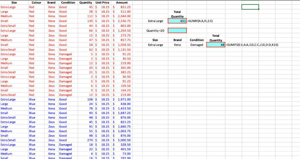
In the spreadsheet above:
=SUMIF(A:A, I5, E:E)
This finds all rows where the Size is “Extra Large” and adds up the Quantity from column E.
Giving you the answer: 651 units
The next formula, =SUMIFS(E:E, A:A, I10, C:C, J10, D:D, K10), goes more in depth and summing up rows where
- Size = Extra Large
- Brand = Xena
- Condition = Damaged
Giving you the answer: 48 units
CountIF Use Case Example:
Managing guest lists might seem simple, until you’re juggling dozens of names, dietary requirements, and attendance statuses. That’s where Excel’s COUNTIF and COUNTIFS formulas become indispensable tools.
Imagine you’re planning a company event with over 30 invitees. You need to know:
How many people have replied?
- Who’s actually attending?
- How many guests require halal meals?
- Who hasn’t responded yet?
- Manually counting these values is time-consuming and error-prone. Instead, Excel does it instantly.
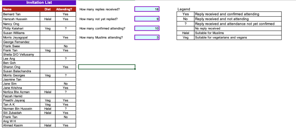
What Excel is doing in this sheet:
| Question | Formula Logic | Outcome |
| How many replies received? | Count any cell in the “Attending?” column that isn’t blank | =COUNTIF(range, “<>”) |
| How many did not reply | Count blank cells (no response yet) | =COUNTBLANK(range) |
| How many are confirmed attending | Count “Yes” responses only | =COUNTIF(range, “Yes”) |
| How many Muslims are attending | Count rows where Diet = “Halal” and Attending = “Yes” | =COUNTIFS(DietRange, “Halal”, AttendingRange, “Yes”) |
With just a few simple formulas, you get instant, error-free answers to key planning questions.
How to Strengthen Your Advanced Excel Skills
If you’re not yet confident with the Excel techniques discussed in this article, don’t worry. Building proficiency takes time, and there are many flexible ways to grow your skills.
- Learn at your own pace
Start by exploring free online guides, articles, and video tutorials that break down complex functions into step-by-step actions. This is especially helpful when you’re trying to understand formulas or visualise how tools like PivotTables or SUMIFS behave in real datasets.
- Observe and learn from others
Shadow a colleague or friend who uses Excel regularly in their role. Real-world exposure to how Excel is used for reporting, analysis, or operations can give you practical insights that aren’t always covered in tutorials.
- Add it to your professional development plan
Committing to Excel as part of your Personal Development Plan (PDP) helps keep you accountable. Whether you’re reskilling, returning to the workforce, or preparing for a promotion, consistent progress with Excel can give you a clear advantage.
- Take a course that suits your goals
The most effective way to build practical, workplace-relevant Excel skills is through structured training.
At James Cook Institute, our WSQ Excel certification courses that are SkillsFuture Credit claimable walk you through real examples, from foundational formulas to advanced spreadsheet functions.
You’ll receive guided practice, direct feedback, and hands-on support so you can confidently apply what you’ve learnt at work.
Explore our Excel courses and take the next step in your Microsoft Excel skills journey