VLOOKUP is an Excel function that helps professionals search for specific information within a spreadsheet by matching a value in one column and returning related data from another column in the same row.
Many professionals use it to organise, connect, and extract relevant data efficiently, whether in HR records, financial reports, or inventory systems. If your role involves working with data in Excel, learning how to use VLOOKUP can save time and reduce errors
Key Takeways:
- Learn what the VLOOKUP function in Excel does and when to use it
- Understand each argument in the formula: lookup_value, table_array, col_index_num, and range_lookup
- See step-by-step examples of VLOOKUP in action using real data scenarios
- Get practical tips on using absolute references and avoiding common #N/A errors
If you’re still building your foundation, our beginner-friendly WSQ Workplace Productivity Using Excel course at James Cook Institute is a great place to start
What is VLOOKUP in Excel
Excel VLOOKUP is useful when you’re working with large datasets across multiple sheets, like pulling an employee’s department from a master list based on their ID. VLOOKUP looks down the first column of a table (hence the “V” for vertical), finds a match, and retrieves a value from a different column in the same row.
VLOOKUP Arguments

The following outlines the arguments this function uses:
- Lookup_value: This is the value you’re seeking in the data set (first column).
- Table_array: This is the range or table containing the lookup value. The function searches in the leftmost column of this array.
- Col_index_num: This is an integer showing the column number within the table where you want to perform the search or retrieve the return value.
- Range_lookup: Determines match type. Use TRUE for an approximate match, or FALSE to return an error if no exact match is found.
Example and Formula of VLOOKUP
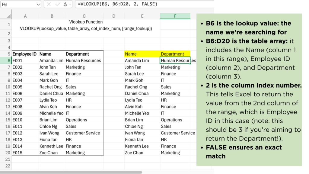
=VLOOKUP(E6, B6:D20, 3, FALSE)
1. Lookup_value – E6
This is the value you want to look up. In this case, E6 contains the employee’s name, for example, “Amanda Lim”.
This tells Excel: search for the name entered in cell E6.
2. Table_array – B6:D20
This is the range where Excel should search for the name and return the related value.
VLOOKUP always searches in the first column of this range—in this case, column B (Name).
So, the formula searches for the value in E6 within the range B6:B20, and then looks across to columns C and D.
3. Col_index_num – 3
This specifies which column to return data from, relative to the first column of the table array.
Column 1 = Name (B)
Column 2 = Employee ID (C)
Column 3 = Department (D)
So, this tells Excel to return the value from the third column in the range, which is the Department.
4. Range_lookup – FALSE
This tells Excel to look for an exact match only. If it doesn’t find the name exactly as typed in E6, the result will be an error (#N/A).
The formula searches for the name typed in E6, finds it in column B of the range B6:D20, and returns the corresponding department from column D in the same row.
How to use VlookUp in Excel
When using VLOOKUP formulas in real-life worksheets, a helpful best practice is to lock the table array using absolute cell references (like $B$6:$D$20) to keep the range fixed when copying the formula down a column.
The lookup value is typically a relative reference (like A6), so that Excel automatically updates the reference as the formula is dragged down through multiple rows.
Here’s how it works:
- A6 is the cell containing the name you want to look up.
- $B$6:$D$20 is the range where Excel will search. VLOOKUP will always search in the first column of this range (in this case, column B which contains the names).
- 3 tells Excel to return the value from the third column in the range, which is the Email column (column D).
- FALSE ensures that only exact matches will be returned.
Enter the above formula in the first cell under the “Email” column (e.g. B6 on the right side), then drag it down to apply it for the rest of the names. Each row will now return the correct email address based on the employee’s name.
Key Things to Remember about VLOOKUP
- VLOOKUP only searches to the right: The function always looks in the leftmost column of the table array and can only return values from columns to the right. If you need to retrieve data from a column to the left, consider using the INDEX and MATCH (or INDEX and XMATCH in Excel 365) combination instead, which allows for more flexible lookups.
- VLOOKUP is not case-sensitive: It treats uppercase and lowercase letters as the same. If you need a case-sensitive lookup, you’ll need to use a different formula setup designed to handle case distinctions.
- The last argument matters: The fourth argument in VLOOKUP – TRUE or FALSE – controls the match type:
- Use FALSE for exact matches (which is most common).
- Use TRUE for approximate matches
- Approximate match requires sorted data: If you’re using TRUE for an approximate match, ensure that the lookup column is sorted in ascending order. If it isn’t, Excel may return incorrect results.
- #N/A means no match found: When VLOOKUP can’t find the lookup value, it returns a #N/A error. This is normal behaviour and indicates that no exact (or appropriate) match was located.
Final Thoughts About VLOOKUP
VLOOKUP remains one of the most widely used Excel functions, especially for quick lookups across large datasets. Once you understand how each argument works and how to apply the formula correctly, it can save you hours of manual work and reduce errors.
That said, Excel has evolved. If you’re using Microsoft 365, it’s worth exploring functions like XLOOKUP or INDEX-MATCH for more flexibility.
Want to go beyond just knowing the formula? Our Level Up Your Excel course covers intermediate functions like VLOOKUP, COUNTIFS, and more – all designed to help you work faster, cleaner, and with more confidence in real-world scenarios


